
Associated Wikis
(privileges may be required)
User Tools
Sidebar
chara:pavo_analysis_manual
Table of Contents
Preliminaries
Downloading the Pipeline
The PAVO data reduction pipeline is available through the CHARA Git repository. Contact Nils Turner or Fabien Baron if you need an account. The software is also installed on the data reduction machine in Atlanta. Please contact Jeremy Jones if you would like an account to reduce your data there. IDL is needed to run the reduction and calibration scripts.
To download the PAVO software:
git clone https://gitlab.chara.gsu.edu/theo/chara_IDL.git
To update the PAVO software:
git pull
Setting up IDL
In addition to the PAVO code, you will need to download the Goddard astrolib library from http://idlastro.gsfc.nasa.gov/, and put this in your path. Then set up an idl_startup.pro… Mike Ireland does the following (adapt for your own setup if you have other IDL uses).
- Put the astrolib library in ~/code/astrolib. And put other useful stuff (like John Monnier's oifits libraries) also in code. Then add setenv IDL_STARTUP ~/code/idl_startup.pro to your .cshrc file.
- Assuming that you've done the CVS checkout above into ~/, use the following for your idl_startup.pro:
defsysv, '!PAVO_DIR', '~/control/idl/pavo/'
!path = expand_path(' ~/code')   ":"   !path
!path = expand_path(' ~/control/idl/pavo')   ":"   !path
Then everything should work. Alternatively, just create a logical link to ~/control/idl/pavo from ~/code/pavo, and the second !path command isn't needed. A matter of personal style (and easily interacting with other IDL programs you might use).
Data Analysis Strategy
PAVO data is not labelled by distinct dark, on-fringe and off-fringe files. Instead, a program has to go through the file headers and make a mostly human-readable headstrip file. This is not a substitute for good log taking.
Fourier-Based Analysis
In this analysis, the first thing that happens is that each frame is turned into a data cube, with wavelength and 2D pupil position. Then each wavelength is analysed using a 2D Fourier transform, where the power is chopped out, the data inverse-transformed and the analysis done on the demodulated fringes in the pupil-plane.
Demodulation (model-based) Analysis
This is the method used to get group delays in get_gd.pro. There is some potential for this method to deliver improved results for the very faintest 3-telescope data. Consider this to be experimental only. If this is sped up in a later version of the code, the output quantities from processv2.prowill not have to be recalculated. The latest ideas (1 April 2010) are to use Graphics Processing Units (GPUs) in a collaboration with the school of IT at Sydney, with a timescale of late-2010, or sparse matrices. The prototype will be sparse matrices in IDL. If GPUs were to be used (1000 times faster than a PC), then we estimate 2 weeks to analyze all PAVO data taken thus far!
Programs for Analysis
headstrip.pro
Use this program like headstrip, /raid/080921/ to go through the directory and find the important information from the headers. The information is saved in a text file in the directory called headstrip.txt [TODO: add a date to this filename, and make this an automatic part of endnight].
processor.pro
This, or something you name yourself, is an example of how to script multiple data analysis runs.g. over a weekend. It is an excellent way to keep a diary of what was run before. NB You either have to run processor.pro, or a variant of it, in the same directory where processv2.pro and the pavo_default_params files are OR you have to devsysv, '!PAVO_DIR' (see above).
processv2.pro
This is the main program for analysis. Originally, it was only for V2 analysis. These options are all inputs to processv2.pro.
- nohann Usually, a window is applied in the Fourier domain. Setting this keyword means that a window isn't used.
- lambda_smooth This is the very most important option. It specifies the number of n wavelength channels over which signal will be coherently smoothed over to increase S/N by sqrt(n). Can be used for data on faint stars but should be used with caution. At the moment it's probably best to not set lambda_smooth for your first analysis, and check the influence of lambda_smooth if you're not satisfied with the results.
- individual Essential for rejecting bad data.
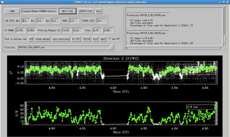
- plot Always use this option when you are running a new data analysis. The plots will look like the following for a strong fringe on baseline 1, which uses beams 1 and 2:
The outputs from processv2.pro are:
- The out_file, which is the text file output, containing V2 values, estimated errors, closurephases etc.
- The .pav files from individual analysis. These are IDL variable files that contain finely sampled V2 and closure-phase.
- The log file, which contains the settings used for the out file.
- If /plot is set, a screenshot of the output of the wavelength calibration will be created. A faulty wavelength calibration has strong potential to screw things up, and it should therefore be checked before proceeding in the analysis. Offsets and Rotation are listed in the log file: Offsets of /- 2 pixels are ok, everything higher should be suspicious. An example plot for an ok wavelength calibration with an offset of 1.2 can be found here (solid line = flux vs lambda after correcting for offset, dashed line = calibrated inflection point of PAVO filter).
l0_l1_gui.pro
This program takes the .pav files and performs an automated outlier rejection as well as enables the user to manually reject bad sections of data. This program can only be run if /individual is set when running processv2.pro (i.e. .pav files have been created), which should really be the default option.
Walkthrough:
1) generate a file which contains the path and names of your .pav files you want to analyse, one .pav file per line. Suppose in the following this file is called list, and an example .pav file is called example0.pav.
2) start the GUI in IDL, click on the LOAD button and load the file list. The output files for all scans will be called list_l0l1.res.
3) The program will start showing results for the first .pav file, with the top panel displaying UT time versus V2, and the bottom panel UT time versus S/N (calculated in real-time (RT), i.e. the number you see in the PAVO server during observing). In the top panel each wavelength is shown as a white dot, and white squares are the average V2 over all wavelengths. Green squares are frames which are kept with the current rejection criteria. A screenshot of this for good 1-bl data can be found here.
4) Outlier rejection is based on 3 criteria: S/N, seconds after lock on fringes is lost (NSEC) and deviation from mean in sigma (SIGMA LIMIT); The default values for this should be fine in most cases; S/N cuts are probably the most sensible to be adjusted if data is particularly bad/good.
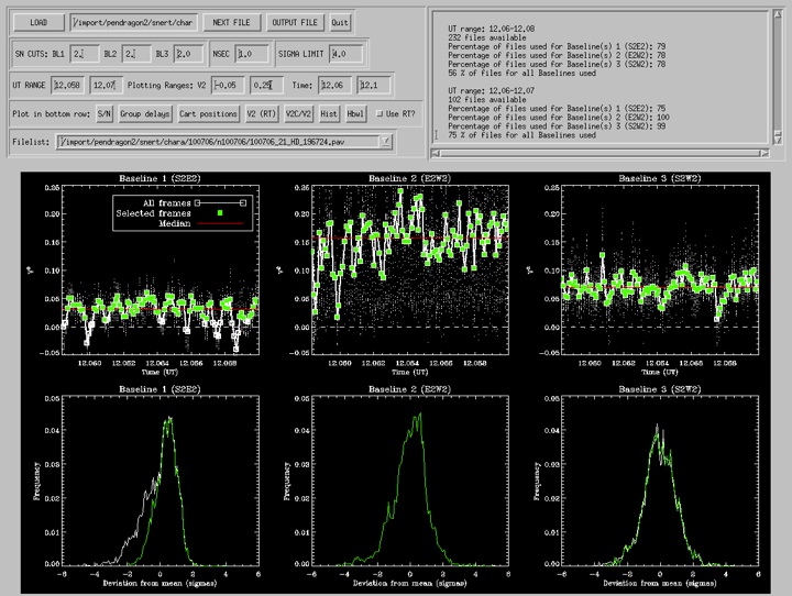
5) The bottom row shows a range of diagnostics that can be used to determine the quality of data such as group delays, cart positions, V2C/V2 (measure of t0, good if high) and histograms. An example for a histogram display for 3-bl data can be found here. The top right window will display the fraction of datapoints rejected with the current settings.
6) Once you're satisfied with the rejection settings for the scan press OUTPUT FILE, which will show V2 vs lambda using all frames that survived the outlier rejection. This step will create and entry in the output file list_l0l1.res, as well as an individual file example0.pav_UT??_UT??.dat, depending on the UT range that goes into the scan.
Note: If you are adjusting outlier rejection criteria, it is probably a good idea to use a set of best settings for all scans of a single night (rather than adjusting them star-by-star) in order to avoid bias in your calibration. Ideally you shouldn't have to adjust anything, and simply use the graphical inspection to decide which scans are useful for calibration and which are not.
Note2: OUTPUT FILE also create additional files called example0.pav.ind and example0.pav.cov. The contain the array indices of frames that are kept for each file, as well as the covariance matrix of each scan which are used in l1_l2_gui.pro
l1_l2.pro
This program takes as input the out file from processv2.pro and the telescopes in use, and calibrates the visibility data. Some key options for this are:
- diamsfile This is an optional text file with two columns. The first is the star name (exactly as in processv2.pro) and the second is the angular diameter of the star. This feature hasn't really been tested, needs diameter errors and correct propagation (anyone?).
- exp If you turn this feature on with /exp, the photometry is used to correct the visibilities for photometric fluctuations. Definitely at least try it for 3-telescope data. Sometimes, 2-telescope data seems to be more stable than the photometric measurements themselves: hence this is an option rather than the default.
l1_l2_gui.pro
A GUI extension of l1_l2.pro to calibrate data, including multi-bracket calibration and proper uncertainty calculations using Monte-Carlo simulations. This program can only be run with the output of l0_l1_gui.pro (see above).
Walkthrough:
1) Load the output file generated by l0_l1_gui.pro. If you run the program for the first time it will search for coordinates using querysimbad to calculate projected baselines etc, which takes a few minutes.
2) Load your estimated calibrator diameters using the CAL DIAMETERS button - see diamsfile keyword in l1_l2.pro above. The third column can be used to specify diameter uncertainties for the calibrators. *This step is mandatory for sensible science calibration*
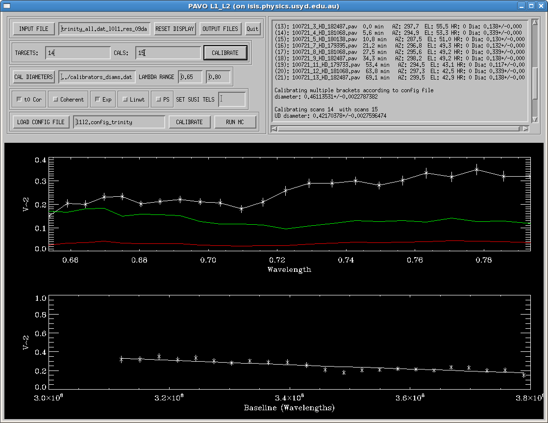
3) Using the TARGETS and CALS boxes in the second row you can calibrate individual scans of data, including averages of multiple scans (separated by a comma in the box). The scan numbers including information on elevation, azimuth, time between scans and expected diameter can be found in the top right box. This feature should be used to identify the brackets that you want to use for the final calibration, and to identify bad calibrators (e.g. by calibrating calibrators with each other). An example screenshot can be found here.
4) Once you have identified the brackets that should be used for calibration, edit the l1l2.config file and specify the brackets by listing the .pav files as shown in the example (note that you need to give the full path to the .pav files if they are not in the same directory). The parameters in the top part of the file are relevant for the Monte-Carlo simulations used to estimate uncertainties. A mandatory parameter to edit here is the estimate for the limb-darkening coefficient of your star (set to 0 if you want a UD fit).
5) Load your config file using the LOAD CONFIG FILE button and press CALIBRATE to perform the multi-bracket calibration. A LD/UD will be performed automatically. Press OUTPUT FILES to output the data of this graph.
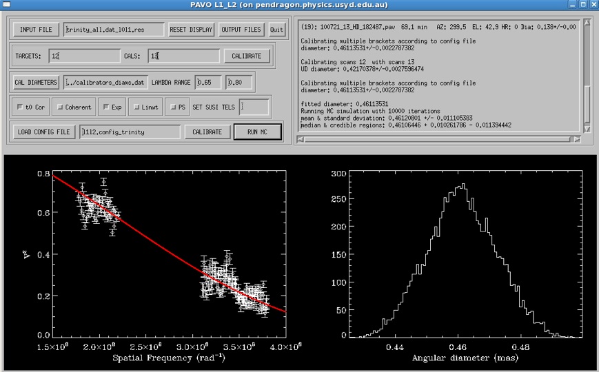
6) Pressing RUN MC will start the Monte-Carlo simulations to calculate uncertainties of the UD fit to the data. The simulations include uncertainties in wavelength scale, calibrator diameters, measurement errors, limb-darkening coefficient and correlations between wavelength channels (see here for an example output screenshot). This feature is so far only implemented for a simple UD fit.
Note: /exp is default in this program as I've found it to improve the calibration in almost all cases.
Nice features to add
processv2: Knowledge of the telescopes from the start, i.e. finding if 2 or 3 telescopes were used based on the shutter sequences.
l1_l2_gui: Add more complex models such as binaries etc in fitting routine.
chara/pavo_analysis_manual.txt · Last modified: 2018/11/29 15:30 by jones
Except where otherwise noted, content on this wiki is licensed under the following license: CC Attribution-Share Alike 4.0 International
