
Adaptive Grid Search for Binary Stars
A set of IDL routines for performing an adaptive grid search for binary stars was written by Gail Schaefer. The program fits a binary model to interferometric data by searching through a grid of binary positions to find a global solution with the minimum chi squared. At each step in the grid, the code uses mpfit to minimize the binary solution. An "adaptive" grid search can be performed where the program adjusts the separation in RA and DEC, as well as the flux ratios at each step in the grid. This is useful for finding the global minimum in the chi2 surface over a wide range of separations. Alternatively, a fixed grid search can be performed to map out the chi2 surface at fixed separation intervals after the best fit solution is found.
The program extracts the squared visibilities, closure phases, and uv coordinates from an OIFITS file. The uv coordinates are used to calculate the visibilities and closure phases for a binary model based on the initial separation, position angle, and flux ratio. The code uses the mpfit package to minimize the binary solution at each step in the grid. The global minimum in the grid is retained as the best fit solution.
Download the IDL Binary Grid Search Software
Download the IDL gridsearch_binary_oifits package here (updated 2025Oct15). Unpack the tar file and include the gridsearch_binary_oifits directory in your IDL path.
Running the binary grid search routine also requires the IDL OIFITS library developed by John Monnier, the IDL mpfit package developed by Craig Markwardt, and the IDL astronomy library maintained by NASA Goddard Spaceflight Center. These packages can be downloaded through the following links:
- Download the IDL OIFITS Library (both OI_DATA and OI_FITTING)
- IDL Astronomy Library (including the Coyote Graphics Library)
Starting the IDL Program
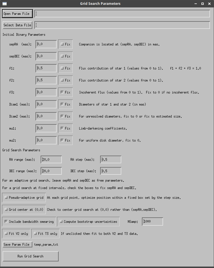
Running the gridsearch_binary_oifits_gui routine will bring up a graphical user interface (GUI) where the user can enter the initial binary parameters and search ranges directly into the GUI. Alternatively, these values can be loaded from a formatted text file (see sample parameter file). If the values are entered into the GUI by hand, make sure to hit enter after typing in the values in each box so that they are registered by the GUI. Each parameter and option is discussed in more detail below. After entering all of the parameters, click the "Run Grid Search" button to begin the binary grid search.
IDL> gridsearch_binary_oifits_gui
OIFITS Data File:
The OIFITS data file containing the interferometric measurements (visibilities and closure phases) can be selected using the "Select Data File" button.
Binary Star Parameters:
The initial values for the binary star parameters can be entered by hand or read from a text file by using the "Open Param File" button. The format of the text file is given in the sample parameter file. Any of the binary star parameters can be held fixed by clicking the "Fix" box next to each parameter. For an adaptive grid search where the binary position is optimized at each step in the grid, then leave sepRA and sepDEC as free parameters. For a grid search at fixed intervals where the binary position is held fixed at each step in the grid, then check the boxes to fix sepRA and sepDEC.
- (sepRA, sepDEC): Binary separation projected into RA and DEC in mas.
- f1: Fractional flux contribution of the primary (values range from 0 to 1).
- f2: Fractional flux contribution of the secondary (values range from 0 to 1).
- f3: Fractional contribution of incoherent flux (e.g., amount of light from a wide companion that is outside of the interferometric field of view). Values range from 0 to 1. If the system is a simple binary with no incoherent background flux, then fix f3 = 0.
- NOTE - The total normalized flux sums to unity: f1 + f2 + f3 = 1.0
- diam1: Angular diameter of primary in mas. For an unresolved diameter, fix the diameter to 0 or fix to the estimated size.
- diam2: Angular diameter of secondary in mas. For an unresolved diameter, fix the diameter to 0 or fix to the estimated size.
- mu1: Limb-darkening coefficient for primary. For a uniformly bright disk, fix the coefficient to 0.
- mu1: Limb-darkening coefficient for primary. For a uniformly bright disk, fix the coefficient to 0.
Grid Search Parameters:
- Range and step sizes for the separations in RA and DEC (in mas).
Options:
A few additional options are available for defining the grid search parameters.
- Pseudo-adaptive grid search: Checking this option will perform a pseudo-adaptive grid search where the binary separation at each grid point is allowed to vary within a fixed box set by the step size. This option is useful if there are multiple solutions possible in the chi2 surface. It allows one to perform a large grid search using a course step size without the risk of skipping over a significant solution in a completely fixed grid. In a regular adaptive grid search, the optimized solution might wander outside of the step size, so the final chi2 map containing the best fit solutions might be sparsely sampled. The pseudo-adaptive grid search will provide finer sampling with the flexibility of finding the best fit within each step.
- Grid center at (0,0): Check this option to fix the center of the grid search at the location of the primary (0,0). This option is useful if the best fit position of the companion is entered as the initial binary parameters and you want to explore the chi2 surface symmetrically on both sides of the primary.
- Include bandwidth smearing: Check this box to include bandwidth smearing to account for the spread of wavelengths across the filter bandpass (or width of the spectral channels). This is particularly important when the separation of the binary is near the same size as the coherence length of the filter (λ2/Δλ). Monochromatic light can be assumed by unclicking the "Include bandwidth smearing" button.
- Compute bootstrap uncertainties: Check this box to compute bootstrap uncertainties and enter the number of bootstrap uncertainties into the Nsamp box.
- Fit_V2_only and Fit_T3_only: Click either of these buttons to fit the binary model to only the visibilities or only the closure phases. If these options are not clicked, then the routine performs a simultaneous fit to both the visibilities and the closure phases. This is useful to see whether a fit to different observables gives the same solution. If not, it could indicate possible systematics in the data calibration.
- Save Param File: Click this button to save the initial parameters and search ranges to a text file called temp_param.txt. This file can then be loaded by clicking the "Open Param File" if the code needs to be run again using the same search parameters.
Output - Results and Plots
The global best fit binary solution and chi2 values are output to the terminal window. These values are also saved to a text file called temp_results. A map of the chi2 surface is saved to a file called temp.eps. Several plots are saved showing the uv coverage and comparisons of the measured and modelled visibilities and closure phases.
- temp.eps: A plot of the chi2 surface generated from the grid search routine. The plot shows the chi2 value for the optimized solution at each step in the two-dimensional grid. The large red, orange, yellow, green, blue, purple, and black symbols show solutions within the 1, 2, 3, ..., 7 sigma confidence interval (corresponding to a difference in chi2 of 1, 4, 9, ..., 49). The small black circles show solutions where the difference in chi2 is greater than 49.
- filename_vis2_big.eps: Squared visibilities vs. spatial frequency for the data (black circles with error bars) and the best fit binary model (red crosses). All measurements are plotted on a single plot.
- filename_vis2.eps: Squared visibilities vs. spatial frequency for the data (black circles with error bars) and the best fit binary model (red crosses). The visibilities measured for each baseline are plotted in separate panels.
- filename_t3.eps: Closure phases vs. wavelength for the data (black circles with error bars) and the best fit binary model (red crosses). The closure phases for each closure triangle are plotted in separate panels. This plot is useful for beam combiners with multiple wavelength channels.
- filename_t3_bline.eps: Closure phases vs. maximum baseline in the closure triangle for the data (black circles with error bars) and the best fit binary model (red crosses). All measurements are plotted on a single plot. This plot is useful for beam combiners that measure fringes across a single broadband filter.
- filename_uv_lam.eps: (u,v) coverage of the measurements plotted in units of spatial frequencies (wavelength dependent).
- filename_uv.eps: (u,v) coordinates of the projected baselines in meters (wavelength independent).
- temp_boot.eps: Bootstrap distributions for (sepRA,sepDEC) - if computing bootstrap uncertainties.
In each plot, filename corresponds to the base name of the oifits file (without the .oifits or .fits extension included). A series of IDL arrays are also saved that contain the results from the grid search: ra_array.idl, dec_array.idl, f1_array.idl, f2_array.idl, f3_array.idl, chi2_array.idl. These arrays can be used to re-create the chi2 surface maps plotted using the auto_plot_chi2_binary_radec_scale.pro routine.
Example - Adaptive Grid Search
This section provides an example of how to run an adaptive grid search using CHARA MIRC data obtained on sigma Orionis on UT 2011Sep29. Sigma Orionis is a triple system. The wide component has an orbital period of 160 years and a separation of 263 mas. The close companion has an orbital period of 143 days and a separation of 4.3 mas. The wide component lies outside of the interferometric field of view and contributes only incoherent light to all but the shortest baselines. On the shortest baselines (e.g., S1-S2 with a baseline length of 34 m), light from the wide component adds coherently to produce additional periodic variations in the visibilities and closure phases. For the purpose of this example, we will fit a constant amount of incoherent flux on all baselines. In their final analysis, Schaefer et al. (2016), excluded from the fit the S1-S2 baseline and all closure triangles that included both the S1 and S2 telescopes.
Download sample OIFITS file on sigma Orionis.
Download sample initial parameter file.
Start grid search procedure and load (or enter) the default starting values into the GUI:
IDL> gridsearch_binary_oifits_gui
In this case, the grid search starts by assuming that the primary and companion are both located at (0,0) with equal flux contributions (f1 = 0.5, f2 = 0.5) and no incoherent flux (f3 = 0). The grid search is performed over separations of +/- 10 mas with a step size of 0.2 mas.
Clicking the "Run Grid Search" button will print the initial starting parameters to the terminal window. If these look good, then hit enter to continue. The code takes a while to run, depending on the search ranges and step size.
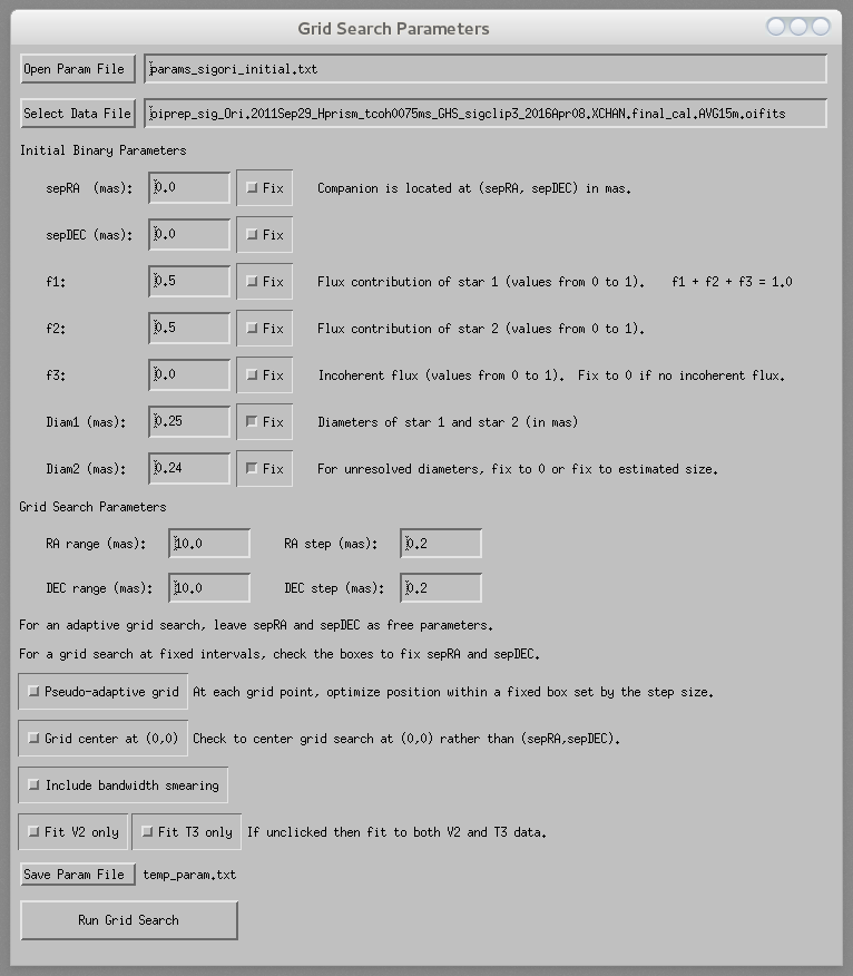
IDL> gridsearch_binary_oifits_gui
---------------------------------------------------------------
Datafile: OIFITS/oiprep_sig_Ori.2011Sep29_Hprism_tcoh0075ms_GHS_sigclip3_2016Apr08.XCHAN.final_cal.AVG15m.oifits
Initial Parameters:
sepRA 0.0
sepDEC 0.0
f1 0.5
f2 0.5
f3 0.0
diam1 0.25 F
diam2 0.24 F
Search ranges:
RA range 10.0
RA step 0.2
DEC range 10.0
DEC step 0.2
Centering grid search at (sepRA,sepDEC)
Assume monochromatic light.
Fitting V2 and T3 data.
Hit enter to continue.
:
...
...
[Initial and final positions of each grid search iteration are printed to the screen.]
...
...
---------------------------------------------------------------
Data file:
OIFITS/oiprep_sig_Ori.2011Sep29_Hprism_tcoh0075ms_GHS_sigclip3_2016Apr08.XCHAN.final_cal.AVG15m.oifits
Best fit total(resid^2) from mpfit:        1803.9789
All chi2:       1803.9786         440       4.1470772
V2 chi2:       878.66771         200       4.5059883
T3 chi2:       925.31088         240       3.9374931
Number of free parameters:           5
Parameter Error
sepRA        -2.7697215    0.0019561813
sepDEC       -5.6180515    0.0025000789
f1           0.43013196    0.0036468646
f2           0.25681558    0.0025902293
f3           0.31305246      -0.0000000
diam1        0.25000000      -0.0000000
diam2        0.24000000      -0.0000000
Close pair separation:         6.2636937 +/-     0.0024034312
Close pair position angle:        206.24348 +/-      0.018969441
Close pair fratio (f2/f1):       0.59706231 +/-     0.0078669841
Flux ratio of wide component relative to primary:       0.72780561
Error ellipse - major, minor, PA:    0.0026240547    0.0017864425       155.50082
Wavelength correction factor:  1.0000    -- No wavelength correction
Fit assumes monochromatic light.
Fitting V2 and T3 data.
When the program finishes, a summary of the results are printed to the screen. This includes the chi2, number of degrees of freedom, and reduced chi2 based on all data, only the visibilities, and only the closure phases. The line reporting the "Best fit total (resid^2) from mpfit" will be consistent with which parameters were fit during the grid search (in this example, both the visibilities and closure phases were fit). The best fit solution from the global grid search are listed (sepRA, sepDEC, f1, f2, f3, diam1, diam2) with errors determined from the diagonal elements of the covariance matrix scaled by the value of the reduced chi2. Fixed parameters will report uncertainties of 0. The amount of incoherent light (f3) is tied to f1 and f2 (f3 = 1.0 - f1 + f2), so an error is not reported directly for that parameter by the mpfit routine.
Below the final parameters, the total separation and position angle measured east of north is reported, along with the flux ratio of the two components (f2/f1). Depending on the uv coverage obtained during the observations, the uncertainties in sepRA and sepDEC might be correlated. The full error ellipse, including correlations between sepRA and sepDEC, is reported on the line "Error ellipse" and gives the semi-major axis, semi-minor axis, and position angle of the major axis of the error ellipse. If there is a large difference between the major and minor axes of the error ellipse, then it would be useful to report the size and orientation of the error ellipse.
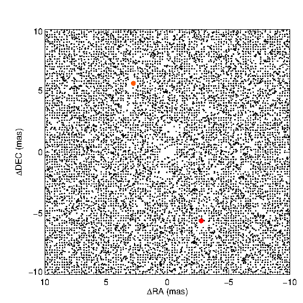
The chi2 surface can be examined in the temp.eps file. The large red and orange circles show the location of solutions within the 1 and 2 sigma confidence intervals (Δχ2 = 1 and 4). The small black circles show much less significant solutions with Δχ2 > 49 found at different points in the adaptive grid search. In this case, the binary solution is very well-defined, with only two realistic possibilities. Actually, these are the same solutions rotated by 180 degree in position angle, with the identification of the primary and secondary flipped. The solution in the south-west has f1 = 0.43, f2 = 0.26, and f3 = 0.31 while the solution in the north-east has f1 = 0.26, f2 = 0.43, and f3 = 0.31.
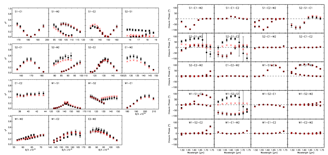
A comparison of the data and the model can be viewed in the other output .eps files. For sigma Orionis, the reason why the periodic binary signature does not reach 1 at the peak in the visibility curves is because of the incoherent flux from the wide component. The discrepancies between the measured and modelled values on the S1-S2 baseline and closure triangles that include the S1-S2 telescopes are because the wide companion is marginally resolved on the shortest baseline.
Example - Fixed Grid Search
The best fit parameters for sigma Orionis on UT 2011Sep29 can be entered as the initial parameters and a finely spaced chi2 map can be generated at fixed intervals. The resulting chi2 map shows the size and orientation of the confidence intervals for the best fit solution.
For a fixed grid search that adequately samples the confidence intervals, the temp.eps file will show contour lines to outline the confidence intervals. As for the adaptive search, the large red, orange, yellow, green, blue, purple and black circles and contours map the 1, 2, 3, ..., and 7 sigma confidence intervals (Δχ2 = 1, 4, 9, ..., and 49). The small black circles show much less significant solutions with Δχ2 > 49.
Computing Systematic Uncertainties from Wavelength Calibration
The following wavelength scaling factors are automatically applied for MIRC-X and MYSTIC (sent by JDM on 2022Aug25):
- Divide all wavelengths for MIRC-X by 1.0054 +/- 0.0006 [Gardner et al 2022]
- Divide all wavelengths for MYSTIC by 1.0067 +/- 0.0007 [Gardner, private communication]
The following wavelength scaling factors are automatically applied for MIRC (Monnier et al. 2012, ApJL, 761, L3):
- Multiple all wavelengths by 0.995 - based on iota peg Konacki orbit. MIRC4T (before 2011)
- Multiple all wavelengths by 1.004 - for 2011-MIRC6T
Use the fix_comb keyword to set beam combiner when INSNAME keyword is incorrect in oifits headers. This is often case for MYSTIC oifits files:
IDL> gridsearch_binary_oifits_gui,fix_comb='MYSTIC'
Computing Bootstrap Uncertainties
If you select to compute uncertainties through the bootstrap method, the code will select the same number of measurements at random with repetition and then randomly vary the selected measurements within their uncertainties. A binary model will be fit to the new resampled set of measurements (using the best-fit as starting position). This process is repeated for Nsamp number of iterations. The uncertainty ellipse that defines 67% of bootstrap distribution is then computed.
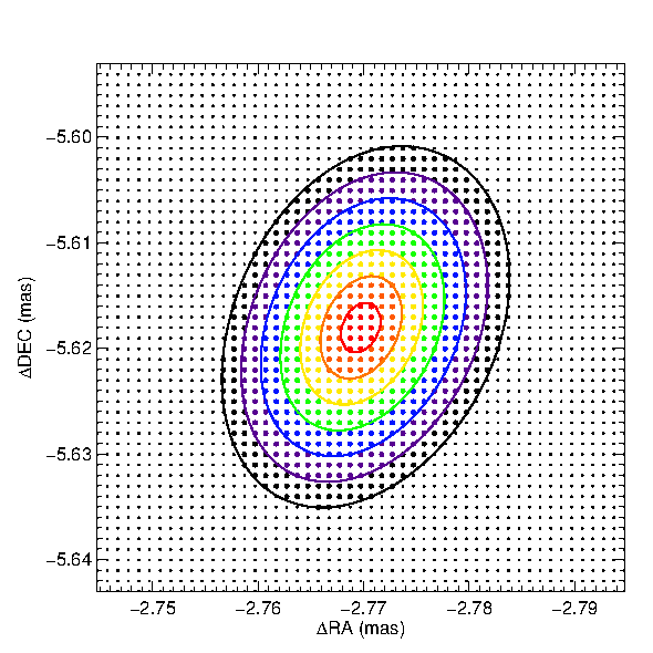
After running through the bootstrap iterations, a plot of the bootstrap distribution in (sepRA, sepDEC) will appear on the screen. If the binary separation is small, the bootstrap iterations might bounce between the two possible solutions on alternate sides of the origin and will skew the statistics to larger uncertainties. The terminal window will prompt the user to ask whether they want to select a specific region to compute the statistics on the uncertainties. The text is shown below - make sure to follow the instructions carefully when selecting regions:
If there are two groups of solutions mirrored about the origin, do you want to select only one solution or trim outliers (y/n)?
: y
---------------------------------------------
You will click on two locations to define the
upper-left and lower-right conrners of a box
that defines the region around the selected
portion of the bootstrap distribution.
STEP 1: Click on upper-left corner:
STEP 2: Click on lower-right corner:
Do you need to redefine the selection region (y/n)?
: n
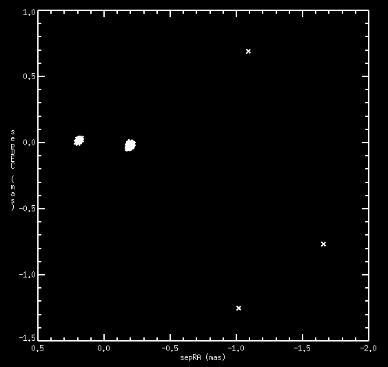
Left: Bootstrap distribution for (sepRA, sepDEC) showing two groups of solutions mirrored about the origin. Right: The box shows the region selected by the user to compute the bootstrap uncertainties.
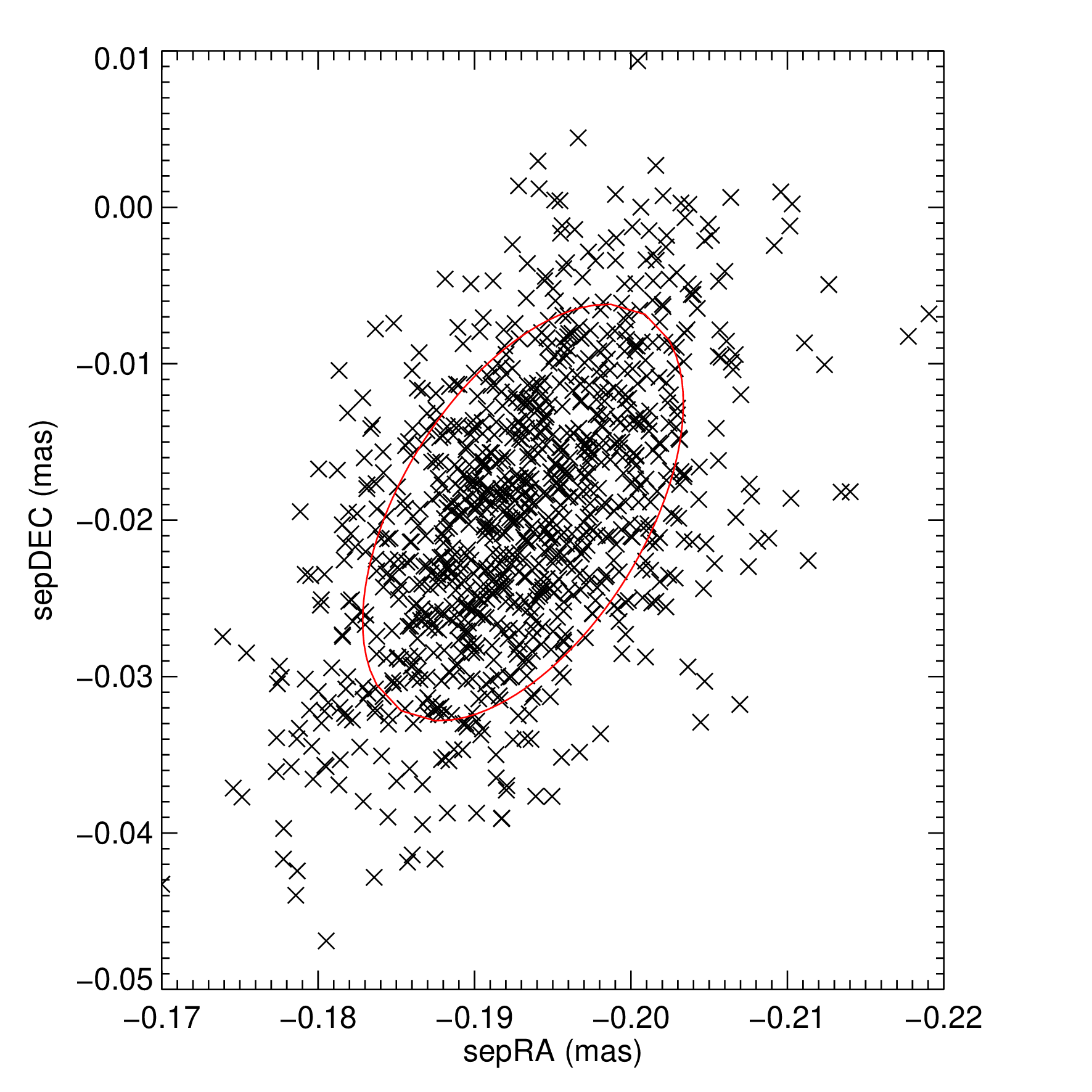
The 67% confidence ellipse confidence interval computed from the bootstrap distribution will be defined on a line that says, "67% confidence ellipse (maj,min,angle)." Compare this to "Total error ellipse - major, minor, PA" computed from the covariance matrix.
Additional Resources
For computing detection limits of faint companions, you might consider using the CANDID companion analysis routine.
Acknowledgments
If you use the IDL binary grid search software in your research, please include the following reference when describing the methods:
Orbits, Distance, and Stellar Masses of the Massive Triple Star σ Orionis - G. H. Schaefer et al., 2016, AJ, 152, 213 (pdf).
Revisions
- 2018Jun05:
- Fixed reading par_yrange from parameter file.
- Turned on QUIET flag when running MPFIT and adjusted format output to screen.
- 2018Jul18:
- Set limits on the angular diameter to be within 0 to 50 mas.
- 2018Aug31
- Fixed plotted errors when plotting only one data point.
- 2018Sep05
- Fixed bounds on sepRA,sepDec when search is not centered at (0,0).
- 2019Jun10
- Correct visibility and phase when passing through null in stellar angular diameter curve.
- 2019Jul31
- Save final results to temp_results in addition to printing to them to the screen.
- Close input parameter file after reading in values.
- 2021Feb25
- Add option to compute uniform or limb-darkened disk diameters for each component. Set limb-darkening coefficient (mu) to 0 for uniform disk.
- For MIRC and MIRC-X data, compute systematic calibration uncertainties in quadrature with formal errors:
5% uncertainty in V2 calibration.
0.5% uncertainty in wavelength scale for MIRC-X (Anugu et al. 2020).
0.25% uncertainty in wavelength scale for MIRC (Monnier et al. 2012).
- 2023Jan19
- Update MIRC-X wavelength calibration uncertainties
5% uncertainty in V2 calibration
0.06% uncertainty in wavelength scale for MIRC-X (Gardner et al. 2022; Monnier priv. comm. 2022Aug25)
0.25% uncertainty in wavelength scale for MIRC (Monnier et al. 2012)
- Update MIRC-X wavelength calibration uncertainties
- Latest distribution: 2023Mar14
- Include wavelength calibration uncertainties for MYSTIC
5% uncertainty in V2 calibration
0.07% uncertainty in wavelength scale for MYSTIC (Gardner, private communication; Monnier priv. comm. 2022Aug25) - The following wavelength scaling factors are automatically applied for MIRC-X and MYSTIC (sent by JDM on 2022Aug25):
Divide all wavelengths for MIRCX by 1.0054 +/- 0.0006 [Gardner et al 2022]
Divide all wavelengths for MYSTIC by 1.0067 +/- 0.0007 [Gardner, private communication] - The following wavelength scaling factors are automatically applied for MIRC (Monnier et al. 2012, ApJL, 761, L3):
Multiple all wavelengths by 0.995 - based on iota peg Konacki orbit. MIRC4T (before 2011)
Multiple all wavelengths by 1.004 - for 2011-MIRC6T - Add fix_comb keyword to set beam combiner when INSNAME keyword is incorrect in oifits headers
IDL> gridsearch_binary_oifits_gui,fix_comb='MYSTIC'
- Include wavelength calibration uncertainties for MYSTIC
- Latest distribution: 2024May30
- Add GUI selections for computing bootstrap uncertainties.
+ Select measurements at random with repetition.
+ Randomly vary selected measurements within their uncertainties.
+ Refit the binary model (use best-fit as starting position).
+ Repeat for Nsamp number of iterations.
+ Compute uncertainty ellipse that defines 67% of bootstrap distribution.
- Add GUI selections for computing bootstrap uncertainties.
- Latest distribution: 2025Aug13
- If combiner keyword INSNAME is set to MIRCX, check the wavelength to see if really MYSTIC data. If so, set the combiner name to MYSTIC for the wavelength calibration.
- Latest distribution: 2025Oct15
- Set mpfit limits on sepRA and sepDEC to be equal to the specified search ranges.