The resolution of a telescope is set by the size of its primary mirror or lens. The larger the diameter of the telescope, the higher the spatial resolution, improving its ability to see finer details. However, there are physical limitations to how large we can build a single telescope. At a certain point, gravity becomes a significant impediment to the physical structure, compromising the optical precision and alignment.
To overcome these challenges, astronomers build arrays of smaller telescopes that they link together to synthesize a larger aperture telescope. This kind of array of telescopes is called an interferometer. The resolution of an interferometer is defined by the distance between the telescopes, rather than the size of the individual telescopes. Therefore we can build an interferometer that has the equivalent resolution of a single telescope that is hundreds of meters in size.
Instead of taking images of stars, an interferometer records the interference pattern (or interference fringes) created by combining the light from two or more telescopes. Interference fringes are created when light waves interfere constructively; the result is a pattern of alternating light and dark bands. The amplitude of the interference fringes encodes information about the size, shape, and brightness distribution of the star.
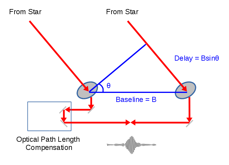
In order to create interference fringes, the star light coming from each telescope has to travel the same distance, down to a fraction of a wavelength (less than 1 micron for optical and near-infrared light). As shown in the illustration below, the light from a star will arrive at one telescope before it gets to another. To compensate for the different distances that the light has travelled to reach each telescope, we send the starlight from each telescope through vacuum tubes into a laboratory. Inside the lab, we equalize the path length by sending the light along optical delay lines. These delay lines consist of movable carts that drive along high-precision rails that continuously adjust their position to keep the telescopes in phase. The starlight is reflected off mirrors on the delay line carts and sent to an instrument that combines the light from multiple telescopes and records the interference fringes on a camera.
What does an interferometer measure?
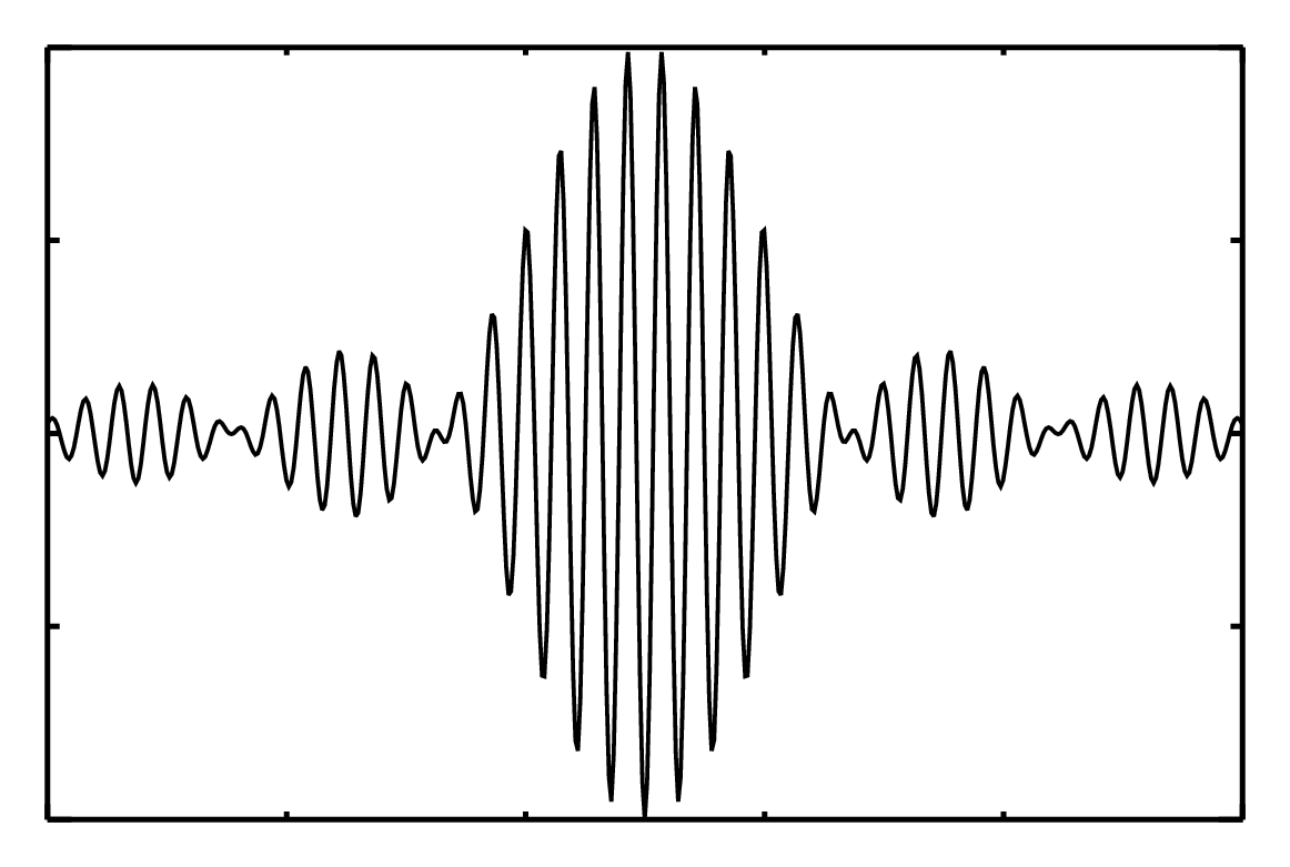
An interferometer records the interference fringes created by combining the light from two or more telescopes. Basic measurements are the amplitude (or height) of the fringes and the phase (or position of the peak in the fringe pattern). The figure below shows an example of interference fringes.
Visibility Amplitudes
The most common measurement in optical and infrared interferometry is a measurement of the amplitude of the fringes. This fringe contrast is often called the "visibility" of the fringes. The normalized visibility amplitude is computed from the maximum and minimum intensity of the fringes, given by
V = (Pmax - Pmin) / (Pmax + Pmin)
An unresolved point source will have high contrast fringes and a normalized visibility amplitude of 1. For a spatially resolved star, light from across the stellar surface combines incoherently causing a decrease in the fringe contrast and therefore, a drop in the visibility amplitude. The normalized visibility amplitude for a resolved source is less than 1. The bigger the star, the smaller the fringes and lower the fringe amplitude. By measuring this drop in the fringe amplitude, astronomers can measure the size, shape, and surface features of a star.
Angular Diameter of a Star
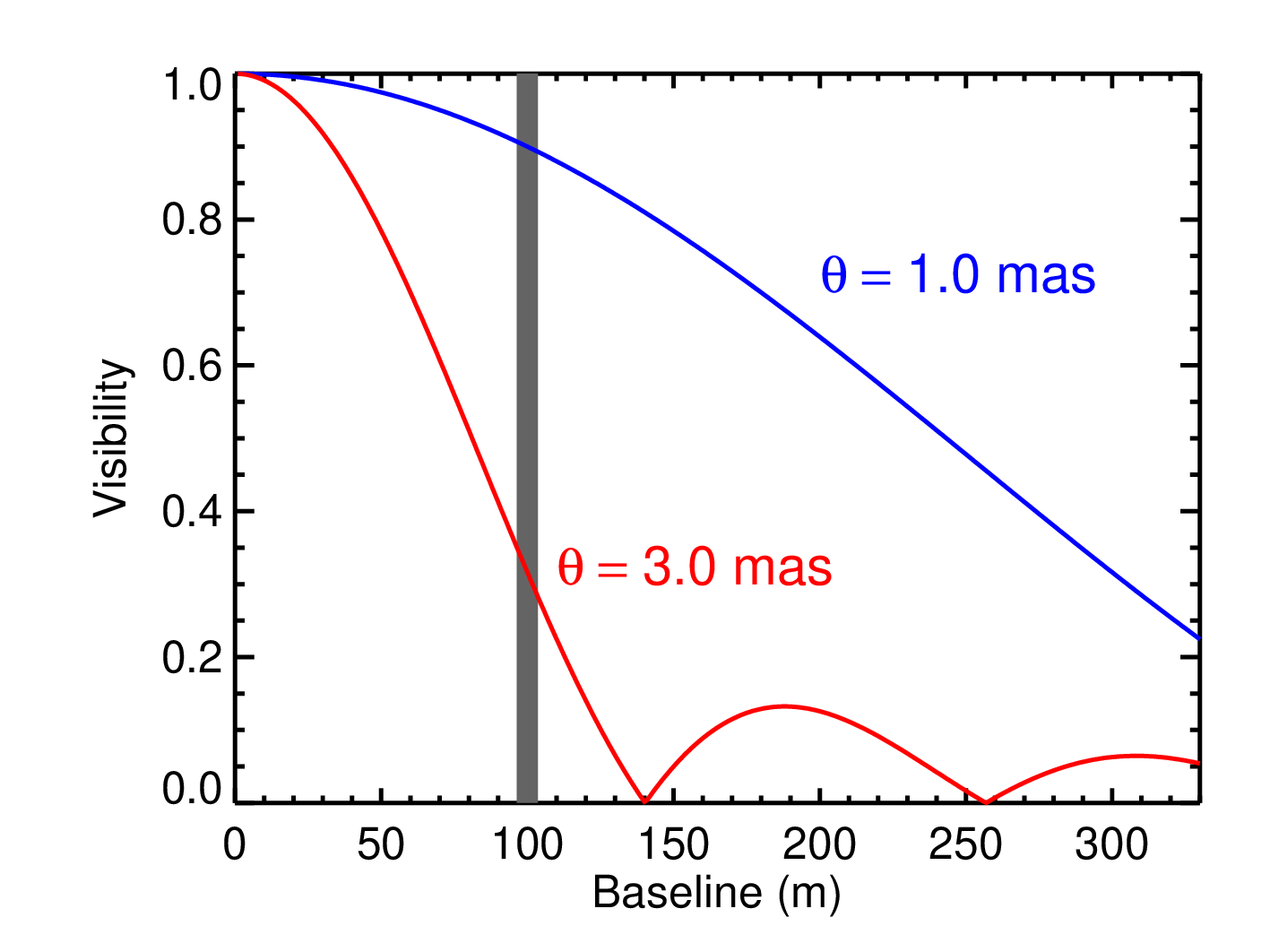
The plot below shows visibility curves for two stars with different angular diameters (measured in milli-arcseconds [mas]). For a given baseline length, a larger star will have a smaller visibility amplitude. The "first lobe" of the visibility curve (before the visibility amplitude reaches zero), contains information about the size and shape of the star. The second and higher order lobes of the visibility curve encode information about the surface features of the star, including limb-darkening, gravity darkening, starspots, and convection cells.
Comparison of visibility curves for a uniformly bright star with an angular diameter of 1 mas (blue) and 3 mas (red).
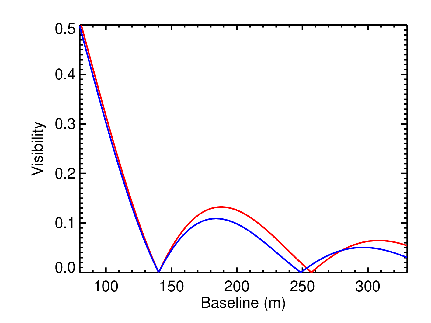
Comparison of visibility curves for a star modeled as a uniform disk and a limb-darkened disk. The effects of limb-darkening are most pronounced beyond the first null.
Binary Stars
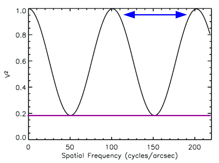
A binary star will produce two fringe packets, one for each star in the system. If the separation between the stars is small enough, the fringe packets from each star will overlap, producing a periodic signal in the visibility amplitudes. An example visibility curve for a binary star is shown in the figure below. The separation between the peaks in the visibility curve provides a measurement of the binary separation while the minimum visibility reflects the flux ratio between the components
Closure Phases
Turbulence in the Earth's atmosphere corrupts the phase of the fringes at optical and near-infrared wavelengths. To recover the phase information, we combine the phases measured in a closed triangle of three telescopes in a way that cancels out the atmospheric turbulence. This quantity is called the closure phase. The closure phase is sensitive asymmetries in the source distribution. A point-symmetric target will have a closure phase of either 0 or 180 degrees (depending on how well the source is resolved). A source that is not point-symmetric will have non-zero closure phases. This includes binaries where the component stars have different brightnesses, a star with a bright or dark spot on the stellar surface, or an asymmetric circumstellar disk around a star. The size the closure phase signal and how it varies across different baselines (or wavelengths) reveals information about the structure of the source.
Differential Visibilities and Differential Phases
Spectrally dispersed fringes produce differential visibilities and differential phases where the visibility and phase of emission lines (like H-alpha or Br-gamma) are measured relative to the stellar continuum. The differential quantities can be used to measure the size and velocity structure of rotating circumstellar disks, outflows, and winds around stars.
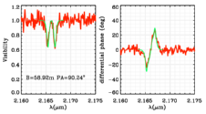
Differential visibilities (left) and differential phases (right) measured for a star surrounded by a circumstellar disk (Meilland et al. 2012, A&A, 538, 110). The drop in the visibility across the emission lines indicate that the disk is more resolved than the stellar continuum. The double-peaked profile corresponds to the blue and red shifted sides of the rotating disk. The S-shaped profile in the differential phase shows a shift in the photo-center across the wavelength channels.