
CLASSIC Data Reduction Pipeline
The CLASSIC / CLIMB data reduction software was written by Theo ten Brummelaar. It is recommended that the code is run using the michelson computer on the mountain or using the Remote Data Reduction machine through the CHARA server in Atlanta. These computers will have the most recent versions of the code installed. The reduction software is maintained through the CHARA gitlab repository. A compiled version of the software is usually available for download on Theo's website. However, this static copy does not always include the most up-to-date version of the code, so it is recommended that the software is run from one of the CHARA computers.
Example CLASSIC data on Kappa Ser from 2018_05_11
The steps below show an example of how to process data using the CLASSIC/JOUFLU reduction pipeline called redfluor. Typing "redfluor -V" at the command line prompt will give the version of the code and list the available options that can be used with the code.
$ redfluor -V
VERSION: V3.2 Fri Nov 12 10:20:28 PST 2021
usage: redfluor [-flags] ir_datafile
Flags:
-a Toggle apodize for FFT (ON)
-A Use shutter sequence A for noise (TRUE)
-b Bootstrap to estimate the Median Error (OFF)
-c Force this to be treated as CLASSIC data (OFF)
-d[0,1,2,3,4] Set display level(1)
-D[Dir] Directory for results (Basename)
-e Toggle edit scans (ON)
-E[min_weight] Edit scans by fringe weight (OFF)
-f Force this to be treated as JOUFLU data (OFF)
-F[env_mult] Change # of envelopes to include (3)
-g Use mean photometry to normalize signal (OFF)
-h Print this message
-H[n] Set percentage definition of high frequency (20)
 Use 0.0 to force using upper integration limit.
-i Toggle manual integration range (OFF)
-I[start-stop] Set integration range of data (AUTO)
-j Toggle adjusting filter width using Vg (ON)
-J Toggle ignoring photometric data (OFF)
-k[0,1] Set method of calculating Kappa (KAPPA_BY_SCAN)
 0 - Calculate for each scan.
 1 - Calculate for total mean.
-l[freq-fwhm] Use low pass instead of Wiener filter (0).
-L Toggle use photometry for noise estimate (OFF)
-m Toggle compute V2 from weighted mean power spectrum (ON)
-M Use weighted mean (ON)
-n Use new data sequence for Fluor (OFF)
-N Toggle correct PS for linear slope after noise subtraction (ON)
-O Toggle Photometry Only (OFF)
-o[n_sigma] Number (float) of standard deviations for outlier removal (OFF, <=0 to turn off)
-p Toggle use postscript (OFF)
-P[smooth_noise_size] Change noise PS +-smooth size (5)
-q Toggle ignore off star data (OFF)
-Q K band shutter background percentage (3.63%)
-R Toggle remote mode (OFF)
-s[spec-chan] Change spectral channel (0=ALL)
-S[smooth_signal_size] Change +-smooth size (1)
-t[start,stop] Truncate scans (OFF)
-u Toggle noise PS multiplier (OFF)
-U Toggle recalculate UV (OFF)
-v Toggle PLPLOT verbose mode (OFF)
-V Toggle REDFLUOR verbose mode (OFF)
-w[freq] Set DC suppression frequency (20.0 Hz)
-x Toggle use dither freq for fringes (OFF)
-X[stddevmult] Set stddev multiplier (0)
-y Toggle use fringe signal for waterfall (OFF)
-Y Toggle use filter for waterfall (ON)
-z[pixmult] Set pixel multiplier (2)
-Z Toggle mean PS for noise estimate (ON)
The README file in the reduceir software package includes a detailed description for these options. Redfluor uses the PLPLOT package to produce the plots it makes, and therefore will also understand any standard Plplot command line arguments. For example, it would be very common to use:
redfluor -dev xwin
on an X windows machine, or
redfluor -dev psc
to produce a color postscript output.
A common way to invoke redfluor is:
redfluor -dev xwin -D/home/schaefer/chara/classic/2018/2018_05_11 -d2 -o3.0 2018_05_11_HD_139087_ird_001.fit
where -D indicates the directory path to save the reduced files, -d2 displays an intermediate amount of plots, and -o3 removes outliers that are more than 3 standard deviations away from the median visibility. The data file to be processed is 2018_05_11_HD139087_ird_001.fit. This command would need to be run for every data file collected.
The first step of the redfluor pipeline will show a waterfall plot of the fringe envelope over time (with time running vertically). On a night of good seeing, the fringe waterfall will be concentrated in the center of the scan window. On a night with bad seeing, the waterfall will look more like a scatter plot, with the position of the fringes bouncing back and forth across the scan window. If there are any gaps in the fringes (vertical regions where the fringes disappear), then these scans should be removed by entering "e" on the command line and clicking on the region to edit.
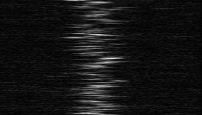
# Processing file 2018_05_11_HD_139087_ird_001.fit
# Vel = 425.0 Lambda = 2.1 BP = 199.2
Move on, zoom in, Zoom out, Edit, Redraw or Clear (m/z/Z/e/r/c)? e
Click on the start of the edit.
Click on the end of the edit.
Move on, zoom in, Zoom out, Edit, Redraw or Clear (m/z/Z/e/r/c)? m
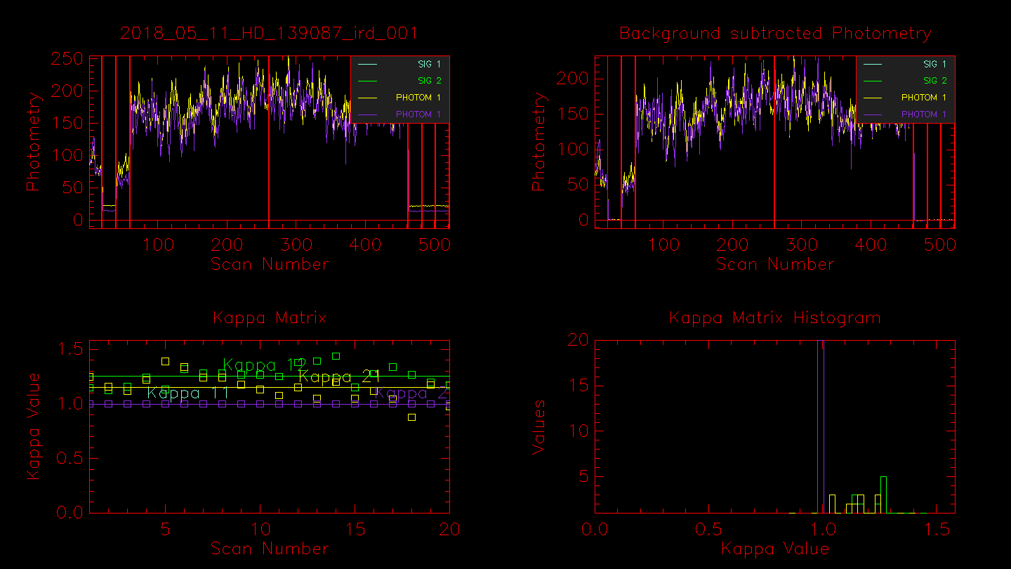
Next the routine will show plots of the photometry (raw and background subtracted). The first three segmented areas show the light from Beam 5, darks (shutters closed), and the light from Beam 6. The next ~ 200 scans are the fringe data (light from both telescopes with fringes). The second set of ~ 200 frames are light from both telescopes but without fringes (carts moved away from the fringe position). The final three segmented areas used to be another shutter sequence, but are now sky frames where the telescopes are moved off the star and the sky background is recorded. The sky frames were added to the observing sequence after it was found that the shutters inside the lab contribute thermal heat in the K-band, which is particularly important when observing faint targets. The last shutter sequence should be checked to make sure that the telescope moved off the star during the sky frames. If you see light during the last sequence and the data were recorded using the new off-fringe and star sequence (e.g., the fits header keyword CC_SEQ = 'OFF_FRG_AND_STAR'), then you will need to run redfluor using the -A flag to use only the first shutter sequence instead.
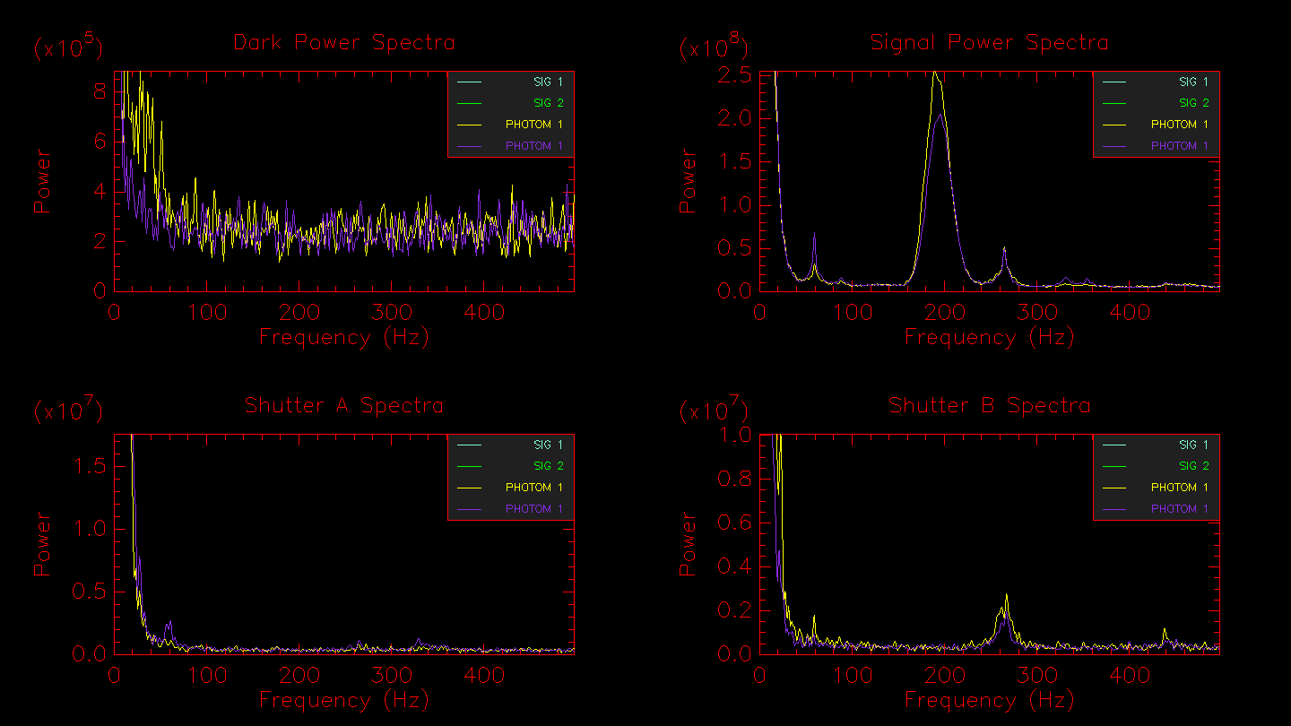
Hitting enter in the terminal window will bring up the next window showing the power spectra for the dark frames, fringe frames, telescope A, and telescope B. In the example below, the fringe peak shows up at 160-240 Hz. Peaks in the dark frames would indicate the presence of electronic noise, whereas peaks in the shutter A or shutter B frames would likely indicate an oscillation of the telescope (e.g., the small peak at ~ 260 Hz in shutter B).
Hitting enter in the terminal window will bring up the next window showing the off-fringe power spectra (light from both telescopes but without fringes), the signal/noise estimate, and the noise subtracted power spectrum of the signal. The noise subtracted power spectrum will also show outlines of the fringe integration regions selected by the Gaussian fit to the fringe peak.
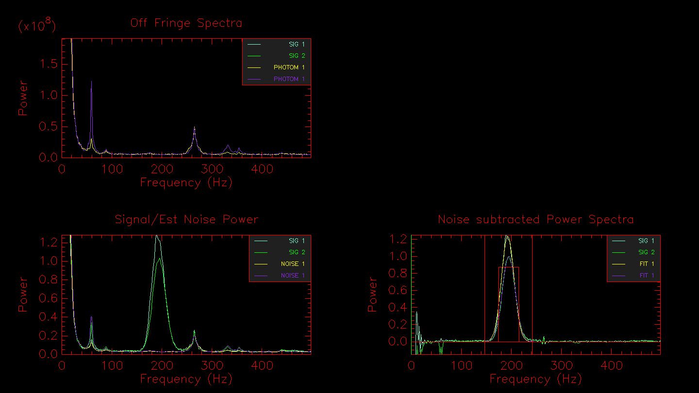
By default, the integration range is set by fitting a Gaussian to the fringe power spectrum peak. If you want to select the integration region by hand, then set the -i flag. Or if you want to define a fixed integration region for all stars in the data set, use the -I[start-stop] flag. The automated integration region will be output to the terminal:
# Vel = 413.9 Lambda = 2.1 BP = 194.0 (193.0, 195.1)
# To get this integration range use
# -I146.82-241.30
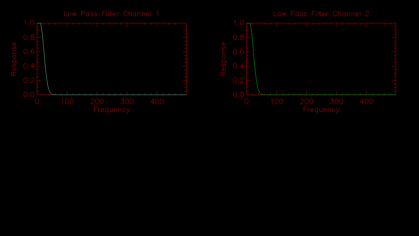
Next is a plot of the low pass filter used to normalize the fringe signal.
Next the routine applies the sigma clipping algorithm if the -o flag is set. The results from the outlier rejection are displayed. If any data points are rejected they will be removed from the plot on the right.
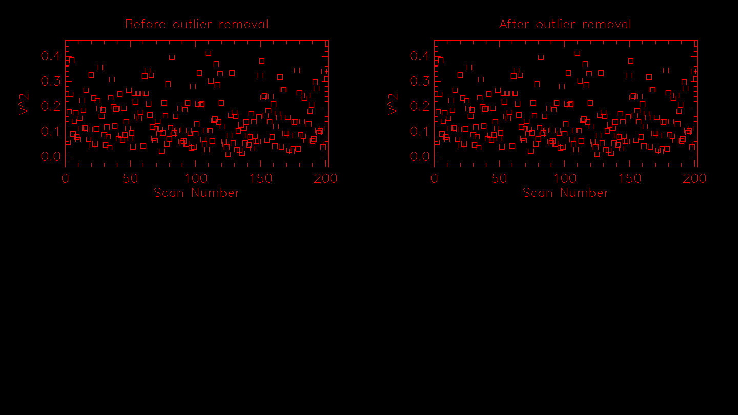
# Calculating .........
# Rejected 0 scans due to low photometry.
# Rejected 0 scans due to being too close to the edge.
# Rejected 0 scans due to low weight.
The next plot will show histograms of the correlation and the fringe weights, the fringe waterfall, and the power spectra waterfall.
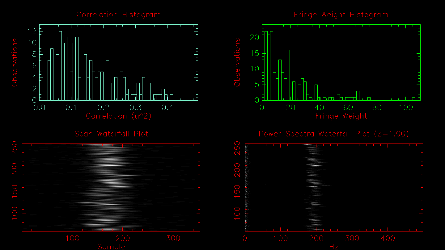
# Results from FLUOR PS calculation method:
N_SCANS	201
#               Mean    Stddev
FRINGE_WEIGHT	17.0262	16.687727
#                  Detector 1     Detector 2      Combined
#               Mean    StdDev  Mean    StdDev  Mean    StdDev
Vg		404.500	14.914	407.346	14.683	405.985	14.860
T0_SCANS		22.8		23.1		22.8
T0_500NM		4.0		4.1		4.0
V2_SCANS	0.23061	0.09691	0.22202	0.10360	0.20814	0.09328
V2_CORR		-1.28396
V2_CHI2		0.00161 0.00368
V2_SQRT		0.48022	0.20180	0.47119	0.21987	0.45622	0.20446
V_SCANS		0.46840	0.10612	0.45678	0.11592	0.44328	0.10813
V_NORM		0.46930	0.16916	0.45788	0.18314	0.44437	0.17075
V_LOGNORM	0.47060	0.09563	0.45978	0.10306	0.44595	0.09627
V2_MEDIAN	0.15592	0.09842	0.14831	0.09635	0.13216	0.09607
V_MEDIAN	0.39487	0.12535	0.38511	0.14176	0.36354	0.13971
Move on, toggle Log, zoom in, zoom out or zoom = 1 (m/l/z/Z/1)?
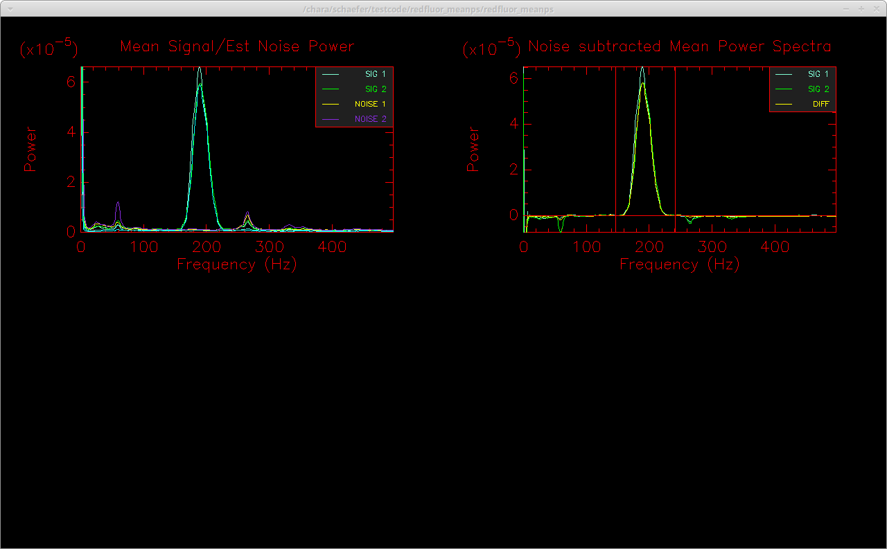
The results for a variety of visibility estimators are printed to the screen. Hitting enter in the terminal window will bring up the final window showing the normalized mean power spectrum of the signal and the noise on the left and the noise-subtracted mean power spectrum on the right. In addition to the visibility estimators listed above, the code will also compute the visibility from the mean power spectrum rather than taking the mean of the visibilities computed from individual scans as done above. This can improve the noise subtraction, particularly for low S/N data. The uncertainty in the visibility of the mean power spectrum is computed through a bootstrap approach. The bootstrap loop can take a few minutes to run, so if you are not interested in computing the visibility from the mean power spectrum, you can turn off this visibility estimator by setting the -m flag. The mean power spectrum computation also includes a linear fit to remove any excess noise to flatten the background in the noise-subtracted mean power spectrum. This feature may not work correctly if there are noise peaks near the fringe integration window. This excess noise correction can be turned off using the -N flag. Another useful flag is -U which can be used to set the DC suppression frequency so that frequencies below the specified value are not included when scaling and correcting the noise.
Finished computing visibility from mean power spectrum.
Hit enter to continue.

Calculating bootstrap uncertainties for mean PS...
V2_MEAN_PS	0.21835	0.00855	0.20785	0.00939	0.19931	0.00821
After the bootstrap loop finishes, the results from the mean power spectrum are printed to the screen. The final results from all of the visibility estimators are output to the screen and stored in the .info files in the directory created for each data file. A few of the most useful visibility estimators include:
- V2_MEAN_PS: Visibility computed from the mean power spectrum. This can improve the noise subtraction, particularly for low S/N data.
- V2_SCANS: Weighted mean of the visibilities computed from each scan individually.
- V_LOGNORM: Visibilities computed assuming log-normal statistics which can better represent changes in correlation caused by atmospheric turbulence.
The three sets of numbers listed for each estimator give the visibility and error recorded for pixel 1, pixel 2, and the difference signal. The default is to use the difference signal, however, comparing the values obtained individually from the two readout pixels could provide an estimate of systematic offsets.
After running through all of the data files for a given sequence of measurements, it is often useful to compare the integration ranges determined for each file. This can be done by running the command line routine "extractir INT_RANGE" in the results directory. Extractir will pull the values for the specified keywords from the .info files in each sub-directory. You might decide to process all data files in a given sequence using a fixed integration range using the -I[start-stop] flag in redfluor.
Useful flags in redfluor
The README file packaged with the redfluor code provides a detailed description of the flags. Several flags that might be useful during a standard reduction or while trying to diagnose problematic data sets are described below:
-m: Setting this flag will turn off the loop to compute the visibility from the mean power spectrum. This will significantly speed up the reduction. It can be useful for a quick look reduction to determine the best integration range for a sequence of stars. It is recommended to remove this flag for the final reduction so that the V2_MEAN_PS estimator is computed.
-N: During the computation of the mean power spectrum, by default, redfluor corrects any residual slope in the noise-subtracted mean power spectrum by linearly fitting the noise on both sides of the fringe power spectrum peak. If there are noise spikes near the wings of the fringe peak, this will corrupt the noise correction (see Figure 3 in Technical Report 98). The residual noise correction can be turned off by setting the -N flag.
-w[freq]: This flag will set the DC suppression frequency. The default value is to suppress all frequencies < 20 Hz. If the low-frequency DC peak is much broader, then the suppression frequency can be adjusted using the -w flag (e.g., -w40). If the DC peak extends past the suppression frequency, this can impact the quality of the noise subtraction for the mean power spectrum. (Note: this used to be the -U flag.)
-A: By default, redfluor computes the noise based on the off-fringe scans. If there is no starlight during the off-fringe frames, or if there are noise spikes in the off-fringe frames that are not present in the data scans, then setting the -A flag will determine the noise from the initial shutter sequence.
-D[dir]: Set the directory for the output files.
-d[0,1,2,3,4]: Set the types of plots to display. The default is -d1. The levels are:
- 0 - Display nothing
- 1 - Display a minimal amount of plots. These include the photometry, the mean power spectra, histograms of the results and some waterfall plots.
- 2 - Adds a few more plots concerning calculation of the Kappa matrix and the optimum fringe filters.
- 3 - Plots details of the reduction of each fringe scan. There will be lots of these, but it can be useful for debugging, for example to see that the amount of data being requested and re-centered for each scan is too large or too small, or that the minimum threshold for the photometry is too high or too low.
- 4 - Plot everything above, as well as the so called "direct" method. This is an experimental method that uses the raw fringe power spectra, that is it is not corrected for the photometry, but the photometric signals are used for estimating the background noise power.
-F[env_mult]: Redfluor looks at each scan to identify the center of the fringe packet and takes a small part of the scan around this center for analysis. The size corresponds to a number of theoretical fringe envelope widths as calculated from the wavelength of band-pass of the optical filter. The default envelop multiplier is set to 4. If too many scans are rejected for being too close to the edge, the envelop multiplier should be decreased (e.g., -F3 or -F2). Setting -F0 forces redfluor to use the entire scan.
-g: Redfluor sends the signal through a low-pass filter to compute the photometry for a scan. For low flux data, normalizing the signal using the filtered photometry can add a significant amount of noise to mean PS calculation. Set the -g flag to use the mean photometry (rather than filtered photometry) to normalize signal. This can significantly improve results for low flux data.
-I[start-stop]: Set this flag to use a fixed range for integrating the power spectrum.
-o[n_sigma]: Number of standard deviations for outlier removal.
-M: Visibility estimators are computed using a weighted mean. The weighted mean is used for computing the mean visibility from individual scans (e.g., V2_SCANS) and when computing the mean power spectra (e.g., V2_MEAN_PS). The fringe weights are computed from a ratio of the power on and off of the fringes. The option to use the weighted mean is ON by default and can be turned OFF using the -M flag to use uniform weights.
-U: From the beginning of 2010 through roughly May 18, 2010, there was an error in the CLASSIC/CLIMB server that produced incorrect u,v coordinates in the fits headers. Turning on the -U flag will recompute the u,v coordinates and correct them in the reduced data files.
-X[stddevmult]: This flag can be set to define the standard deviation multiplier that is used to reject scans with low flux. The default multiplier is 0 (e.g., only scans with negative flux values are rejected). The floor for rejecting bad photometry is set by multiplying the standard deviation of the dark frames by the multiplier. The values for the STDDEV_MULT, STDDEV_DARKS, and FLOOR are listed in the .info files. The number of fringe scans and off-fringe scans rejected due to low photometry are also listed in the .info files. Low flux values that are close to 0 can corrupt the fringe and noise power spectra. Setting the multiplier to ~3 sigma might be suitable for rejecting bad photometry on bright stars, but values of ~ 0.5 sigma might be more appropriate for faint stars where the flux is barely above the background counts.
-Z: Visibility estimators like V2_SCANS are based on the mean of the visibilities computed from each of the individual scans. To prevent negative visibilities from being produced by bad background subtraction of low S/N data, the mean power spectrum of the noise is scaled to the low frequency region of the fringe power spectra of each individual scan. It is ON by default and can be turned OFF using the -Z flag. While minimizing the likelihood of negative visibilities, this option sometimes yields systematic differences in the calibrated visibilities derived for both high and low S/N data.
Calibration
After reducing the data, the calibrator stars are used to calibrate the system visibility (loss in coherence caused by the atmosphere and the instrument) and correct the visibilities measured for the science target. There are three options for running the CLASSIC calibration software:
- calibir - This calibrates the science data based on the nearest neighbor calibrators in each Cal1-Obj-Cal2 sequence.
- calibirgtk - A user-friendly interface for calibir that allows the user to select which stars are calibrators and objects and automatically looks up the angular diameters of calibrators through JMMC.
- calibir_linfit: A version of calibir that computes a linear fit to the calibrator visibilities. This is useful when observing in a Cal1-Cal2-Obj-Cal1-Cal2 sequence. It also allows the user to define breaks in the calibration sequence when alignments were done.
Each of these routines is described in more detail below.
calibir
The calibir program reads the INFO files in the processed data directories at the current location. The routine calibrates the science target using the nearest neighbor calibrators observed before and after the science target. If the alignment changes between a calibrator and neighboring science target, then these observations should be moved to different directories to avoid calibrating across a jump in the system visibilities (or use the -J flag to define a time range for the calibration). If NIRO alignments occurred between two calibrators, then it should be OK to calibrate all of the data in one directory since calibir uses only the nearest neighbors.
A common way to call calibir is as follows:
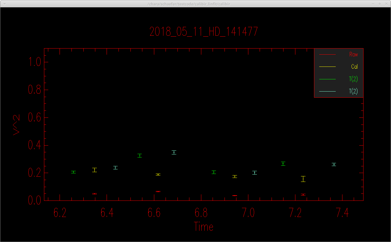
calibir -F -i -s1.1368-0.1069,1.0644-0.1001 -BV2_MEAN_PS HD_141477 HD_139087 HD_142244
where -F saves the output to an OIFITS file based on the name of the object, -i selects objects based on the "ID" name listed in the INFO file, -s sets the calibrator diameters (uniform disk diameters in the K-band of θ = 1.1368 ± 0.1069 mas for HD 139087 and θ = 1.0644 ± 0.1001 mas for HD_142244 estimated by JMMC/Searchcal), and -BV2_MEAN_PS sets the visibility estimator to "V2_MEAN_PS" for both the target and the calibrators. After the flags, the science target ID is listed, followed by a listing of the calibrators in the same order as their diameters in the -s flag. Calibir outputs a plot of the calibrator visibilities (green, blue points), and the raw (red) and calibrated (yellow) visibilities of the science target. In this example sequence, a NIRO alignment was done after every C1-O-C2 set.
By default, the calibrated data are saved to an oifits file with the name 2018_05_11_HD_141477_001.fits. The oifits files can be fit using various data analysis software or read directly into programming languages like IDL.
The full listing of options available in calibir are listed below:
$ calibir -V
Version: V3.1 Mon Jun 10 09:51:29 PDT 2019
usage: calibir [-flags] {OBJ CAL1 CAL2 CAL3...}
Flags:
-b[beta]		Visibility multiplier (1.0)
-B[Vis Type]		Set Vis estimator for Object and Calibrator (V2_SCANS)
-c			Use CHARA number for identifier (OFF)
-C[Cal Vis Type]	Set Vis estimator for Calibrator (V2_SCANS)
-D[spec chan]		Change spectral channel
-f[oif]			Set OIFITS filename (From object)
-F			Toggle saving OIFITS file (OFF)
-h			Print this message
-H			Use HD number for identifier (OFF)
-i			Use ID/Name for identifier (OFF)
-J[mjdmin,mjdmax]	Restrict MJD range (All)
-l			Assumes a linear variation of the cals (OFF). Otherwise also takes into account the cal errors
-n			Use standard error instead of standard deviation (ON)
-N[min_n_Scans]		Minimum number of scans (0)
-o			Invert the sign of the UV coords (OFF)
-O[Obj Vis Type]	Set Vis estimator for Object (V2_SCANS)
-p[detector chan]	Change detector channel (0=diff, 1, 2, 3=weighted mean)
-P{dev}		Toggle plotting, or set device (ON/xwin)
-r			Print raw data (ON)
-s[diam1-err,diam2-err,...]	Size of calibrators in mas (0.0)
-t			Includes variability of the co-Transfer in error.
-S			Self Calibrate mode (OFF)
			If error left out it is set to zero.
-V			Verbose mode (OFF)
-2			Output V^2 table based on V estimator (ON)

Visibility estimators available are:
V_CMB V_FIT V_ENV V_MEAN_ENV_PEAK
V_MEAN_ENV_FIT BINARY_V_A BINARY_V_B BINARY_ENV_V_A
BINARY_ENV_V_B V2_SCANS V_SCANS V_NORM
V_LOGNORM V2_MEDIAN V_MEDIAN V2_SCANS_DIR
V_SCANS_DIR V_NORM_DIR V_LOGNORM_DIR V2_MEAN_PS
If using V2_MEAN_PS as the visibility estimator, then the -n flag (use standard error instead of standard deviation) is automatically turned off in the software. This is because the uncertainty in V2_MEAN_PS is determined from the standard deviation of the bootstrap distribution, so there is no reason to divide by the square-root of the number of scans.
calibir_linfit
The calibir_linfit routine computes a linear fit to the calibrator visibilities when determining the system visibility. This is useful when observing in a Cal1-Cal2-Obj-Cal1-Cal2 sequence, as it will include all of the calibrator observations in the fit (whereas calibir uses only the nearest two calibrators). It also allows the user to define breaks in the calibration sequence when alignments were done. Calibir_linfit uses the same options as calibir. An example of how to call the program is as follows (see description of calibir for an explanation of the flags):
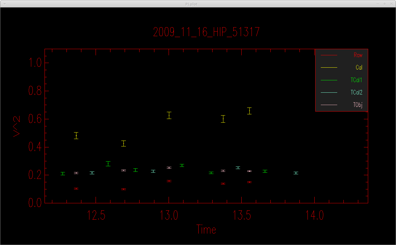
calibir_linfit -i -F -BV2_MEAN_PS -s0.3189-0.0078,0.2553-0.0063 HIP_51317 HD_87301 HD_88725
This will open up a plot showing the raw visibilities of the object and the calibrators.
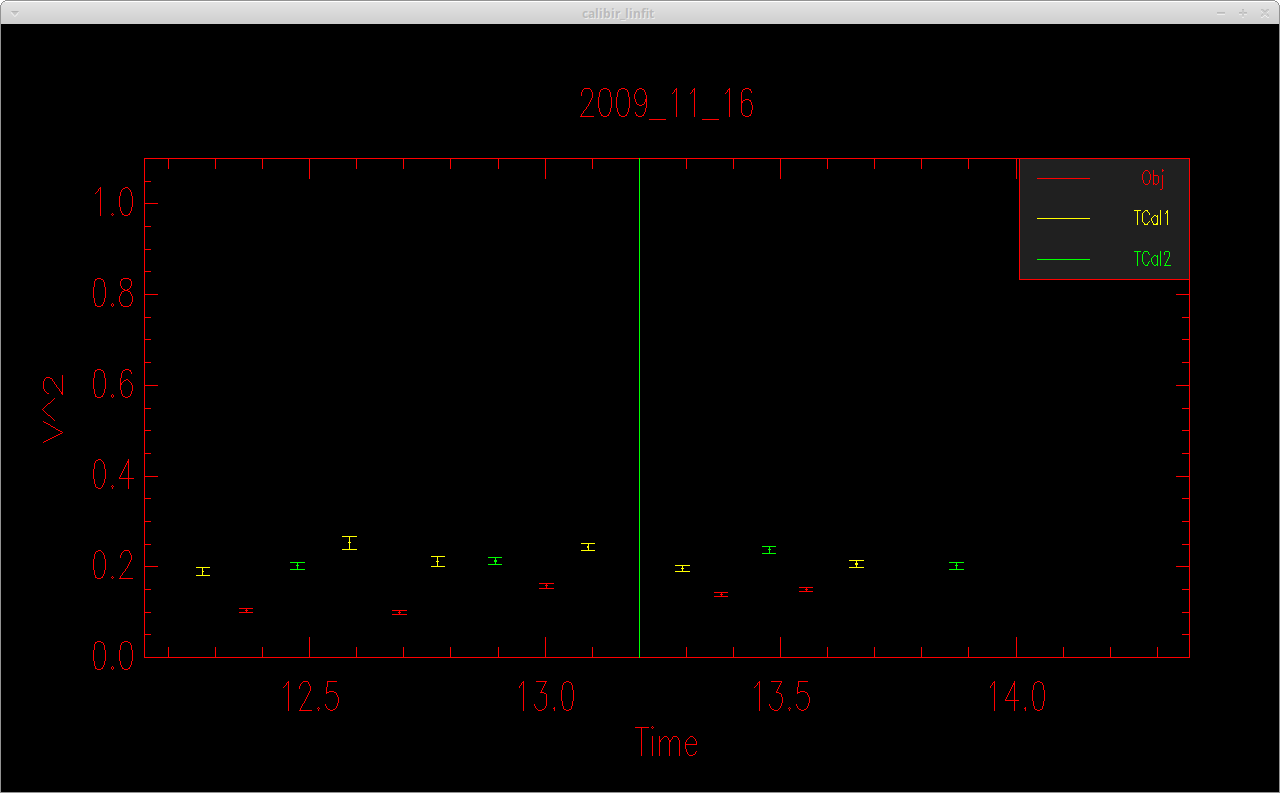
The code will then ask the user if they want to enter a break in the alignment sequence. The user can enter one or more time breaks and a vertical line will appear in the visibility plot at the time of each break.
Do you want to want to define an alignment sequence (y/n)?
y
Enter time of alignment in XX.X hours:
13.2
Time of break 13.20
Do you want to want to define another alignment sequence (y/n)?
n
Hit return to continue.
Number of time breaks: 1
Time break: 0
tmin: 12.27,  tmax: 13.20
Number of CAL observations 6
Number of OBJ observations 3
Time break: 1
tmin: 13.20,  tmax: 13.87
Number of CAL observations 4
Number of OBJ observations 2
The code will then compute a linear fit to determine the system visibility as a function of time for each calibration sequence. It will compute the calibrated visibility of the science target based on the system visibility at the time of science observation based on the linear fit. It will then open a plot showing the calibrated visibilities, print a summary of the results to the screen, and save the results to an oifits file (if the -F flag is set).
calibirgtk
Running "calibirgtk" will open a graphical user interface listing all of the calibrators and objects observed on a given night.
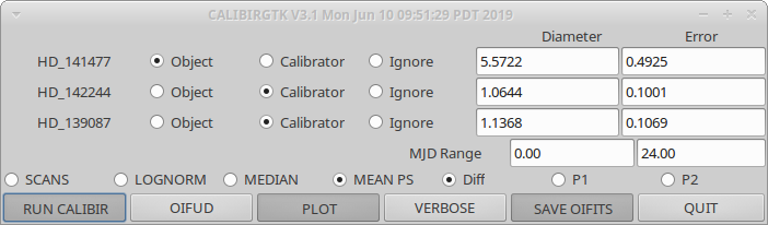
The user can select which stars to use as calibrators, which to use as the science object, or whether to ignore the star. The routine will query the JMMC catalog to look up the estimated angular diameters for each star. These values can also be input by hand into the user interface. Some of the most common visibility estimators (SCANS, LOGNORM, MEDIAN, MEAN PS) are available for selection, as well as whether to use the difference signal, the pixel 1 signal, or the pixel 2 signal. The MJD range can be set if you want to limit the calibration to a smaller subset of the data. Clicking the "SAVE OIFITS" button will save the output to an oifits file.
When the user clicks the "RUN CALIBIR" button, the code will call calibir based on the options selected in the GUI. If the user clicks the "OIFUD" button it will open a dialog box to select an oifits file and run the oifud program to compute a fit for a uniform disk diameter (see below).
By default, calibirgtk calls calibir, the nearest neighbor calibration routine. If you want to run calibirgtk using calibir_linfit, then start the program using the following flag: "calibirgtk -l".
OIFITS Utitlities
The calibrated oifits files can be analyzed using various data analysis software or read directly into programming languages like IDL.
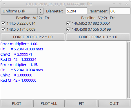
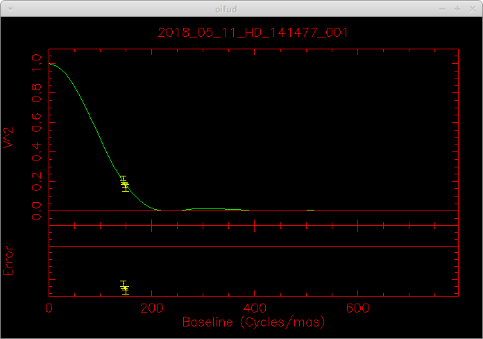
There are a few oifits utilities included in the reduceir package that can be used to manipulate, view, and analyze data. For instance, oifits-merge can be used to merge multiple OIFITS files on the same target (e.g., merge observations from different nights) and oifud can be used to fit simple geometries like a uniform disk to the visibility data:
oifud 2018_05_11_HD_141477_001.fits
Recent Revisions:
- 2018Feb: Use weighted mean of the visibilities computed from the individual scans. The fringe weights are computed from a ratio of the power on and off of the fringes. The option to use the weighted mean is ON by default and can be turned OFF using the -M flag.
- 2019Feb: Modification to prevent negative visibilities from being produced by background subtraction of low S/N data. This option uses the mean power spectrum of the noise scaled to the low frequency region of the fringe power spectra of each individual scan. It is ON by default and can be turned OFF using the -Z flag.
- 2019May: Compute the visibility from the mean power spectrum which will have higher signal than the power spectra of the individual scans. This can improve the noise subtraction, particularly for low S/N data. The uncertainties for the mean power spectrum are computed through a bootstrap approach. The mean power spectrum visibility estimator can be turned off using the -m flag (for faster run times). This feature also includes a linear fit to the background around the fringe peak to remove any excess noise. The excess noise correction can be turned off using the -N flag. The -w flag can be used to set the DC suppression frequency to remove low frequencies from the fit. A detailed description of the mean power spectrum method and examples of how to use this feature are included in the following technical report.
- 2020Jul28: Fixed a bug in the rejection of scans with low flux values.
- 2020Aug18: Add -g option to normalize the signal using the mean photometry rather than the low-pass filtered photometry. This can improve the mean PS calculation for low flux data.
Additional Resources
The CLASSIC/CLIMB Data Reduction: The Math - Theo ten Brummelaar
The CLASSIC/CLIMB Data Reduction: The Software - Theo ten Brummelaar
Using the Mean Power Spectrum to Compute the Visibility with REDFLUOR - Gail Schaefer
CLASSIC J-Band Calibration - Schaefer, ten Brummelaar, Farrington, Sturmann, Anderson, Majoinen, & Vargas